Read your data

Turn a tracking export into an anipoint with aniread, and tell it about your recording.

aniread reads movement data from a wide range of sources: pose estimation from video, centroid trackers, motion capture, even trackball hardware. Whichever tool wrote the file, you get back the same structure, so after this first step it stops mattering.

What it can read

These are the sources aniread supports, with the reader for each and the file types it accepts:

get_supported_sources() |>
  print(n = Inf)

#> # A tibble: 18 x 3
#>    source           reader             suffix   
#>    <chr>            <chr>              <list>   
#>  1 aniframe         read_aniframe      <chr [1]>
#>  2 animalta         read_animalta      <chr [1]>
#>  3 anipose          read_anipose       <chr [1]>
#>  4 bonsai           read_bonsai        <chr [1]>
#>  5 boris            read_boris         <chr [2]>
#>  6 c3d              read_c3d           <chr [1]>
#>  7 deeplabcut       read_deeplabcut    <chr [2]>
#>  8 fasttrack        read_fasttrack     <chr [1]>
#>  9 fictrac          read_fictrac       <chr [1]>
#> 10 freemocap        read_freemocap     <chr [1]>
#> 11 idtrackerai      read_idtracker     <chr [2]>
#> 12 lightningpose    read_lightningpose <chr [1]>
#> 13 movement         read_movement      <chr [2]>
#> 14 octron           read_octron        <chr [1]>
#> 15 sleap            read_sleap         <chr [2]>
#> 16 trackball_bonsai read_trackball     <chr [1]>
#> 17 trackmate        read_trackmate     <chr [1]>
#> 18 trex             read_trex          <chr [2]>

You rarely need to call those readers yourself. read_dataset() reads any of these files: it works out which tool wrote it and calls the matching reader.

Get some data to follow along

You don’t need your own files. get_sample_data() downloads a real export for any supported source and returns its path:

path <- get_sample_data("sleap")

#> Downloading sleap data...

basename(path)

#> [1] "sleap_single-mouse_EPM.h5"

We’ll use this recording in all of the guides: ten minutes of a single mouse on an elevated plus maze, tracked with SLEAP. To see what else is available, call get_sample_data(list_datasets = TRUE).

Read it

movement <- read_dataset(path)
movement

#> # Individuals: individual1
#> # Keypoints:   centre, left_ear, right_ear, snout, tail_base, tail_end
#>    individual  keypoint  time     x     y confidence
#>    <fct>       <fct>    <int> <dbl> <dbl>      <dbl>
#>  1 individual1 centre       1    NA    NA         NA
#>  2 individual1 centre       2    NA    NA         NA
#>  3 individual1 centre       3    NA    NA         NA
#>  4 individual1 centre       4    NA    NA         NA
#>  5 individual1 centre       5    NA    NA         NA
#>  6 individual1 centre       6    NA    NA         NA
#>  7 individual1 centre       7    NA    NA         NA
#>  8 individual1 centre       8    NA    NA         NA
#>  9 individual1 centre       9    NA    NA         NA
#> 10 individual1 centre      10    NA    NA         NA
#> # i 110,900 more rows

What you got back

That’s an anipoint: one row per point (here, each keypoint of each individual) at each moment. It’s one of the aniframe classes defined by anicore, which every other package in the ecosystem reads and returns. Underneath it’s a tibble, so dplyr and ggplot2 work on it as usual. On top, metadata records what each column is for:

Question	Role	Read it with	Here
What is moving?	identity	`get_variables(movement, "what")`	`individual`, `keypoint`
When?	index	`get_index(movement)`	`time`
Where?	position	`get_axes(movement)`	`x`, `y`

get_variables(movement, "what")

#> [1] "individual" "keypoint"

get_index(movement)

#> [1] "time"

get_axes(movement)

#>   x   y 
#> "x" "y"

Two consequences worth knowing from the start:

Column names are free. The roles are what matter, so a file whose identity column is called track works just as well.
The frame arrives grouped by identity, so everything downstream runs within each track rather than across them:

dplyr::n_groups(movement)

#> [1] 6

Six groups: one mouse × six keypoints. That grouping is why interpolation never bleeds from the snout into the tail, and why speed is never computed across the join between two tracks.

Going deeper

This is the short version. anicore’s articles cover the data structure in full: The aniframe data structure for the roles and how to set them, and Metadata on an aniframe for everything below.

Tell it about your recording

An anipoint keeps context that a bare data frame would lose. The reader fills in what the file records:

get_metadata(movement)

#> -- animovement metadata --------------------------------------------------------
#> 
#> -- recording 
#> source: sleap
#> source_version: 1.3.1
#> source_format: h5
#> filename: sleap_single-mouse_EPM.h5
#> 
#> -- time 
#> unit_time: frame
#> sampling_interval: 1 frame
#> 
#> -- space 
#> coordinate_system: cartesian_2d
#> reference_frame: allocentric
#> handedness: right
#> axis_directions: x = right, y = up, z = back
#> axis_extents: y = 861.2433 px
#> unit_space: px
#> unit_angle: rad
#> 
#> -- variables 
#> what   keys: individual, keypoint
#> when   index: time | keys: -
#> where  position: x = x, y = y
#> event  state: - | point: -
#> 
#> -- structure 
#> keypoint: 6 points, 7 segments, 0 joints
#> 
#> Not set: sampling_rate, start_datetime, euler_sequence, euler_intrinsic

Two things are missing that everything downstream depends on: how fast the camera recorded, and how big a pixel is.

Time in seconds

SLEAP’s analysis files don’t record a frame rate, so time counts frames. Declare the rate, then convert the time column to seconds:

movement <- movement |>
  set_metadata(sampling_rate = 30) |>
  convert_unit_time("s")

Use your own frame rate

We’re assuming 30 fps for this sample. Set whatever your recording actually was: everything downstream that involves time scales with this number.

Space in centimetres

Coordinates are in pixels (unit_space: px), which is all a video can tell you. To get real distances you need something of known size in the picture. Here we use the mouse itself: an adult mouse measures about 9 cm from its snout to the base of its tail, and stretched out, this one spans about 140 pixels.

movement <- movement |>
  convert_unit_space("cm", calibration_factor = 9 / 140)

convert_unit_space() rescales every coordinate by that factor and records the new unit. The header now shows the sampling rate and the duration, and from here on, distances come out in centimetres and speeds in centimetres per second:

movement

#> # Individuals:   individual1
#> # Keypoints:     centre, left_ear, right_ear, snout, tail_base, tail_end
#> # Sampling rate: 30 Hz
#> # Time:          00:00:00 to 00:10:16
#>    individual  keypoint   time     x     y confidence
#>    <fct>       <fct>     <dbl> <dbl> <dbl>      <dbl>
#>  1 individual1 centre   0.0333    NA    NA         NA
#>  2 individual1 centre   0.0667    NA    NA         NA
#>  3 individual1 centre   0.1       NA    NA         NA
#>  4 individual1 centre   0.133     NA    NA         NA
#>  5 individual1 centre   0.167     NA    NA         NA
#>  6 individual1 centre   0.2       NA    NA         NA
#>  7 individual1 centre   0.233     NA    NA         NA
#>  8 individual1 centre   0.267     NA    NA         NA
#>  9 individual1 centre   0.3       NA    NA         NA
#> 10 individual1 centre   0.333     NA    NA         NA
#> # i 110,900 more rows

Calibrate against something in the same plane

For your own recordings, film an object of known size, such as a ruler or the arena itself, at the height the animal moves at. A rough scale is fine for following these guides, but measurements are only as good as the calibration behind them.

Take a first look

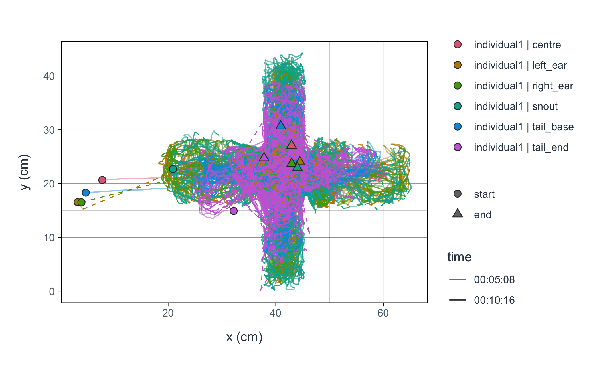
Calling plot() on an anipoint draws the trajectories, with axis labels taken from the metadata:

plot(movement)

Raw SLEAP tracks. The plus maze is clearly visible, and so are a handful of points that landed nowhere near it.

The maze shape comes straight out of the data, with no annotation needed. So do the long lines reaching off to the left: a few dozen points, out of 110,910, that landed well outside the maze. They’re drawn as long straight lines because the plot joins consecutive positions. Whether that matters, and what else is hiding in there, is what the next guide is for.

The skeleton

Pose-estimation tools also record which keypoints are joined to which: the skeleton. SLEAP keeps it in the same file as the tracks, so read_dataset() has already attached it:

get_structure(movement)

#> $keypoint
#> <anistructure> 6 points, 7 segments, 0 joints
#> variable: keypoint
#> Points: snout, left_ear, right_ear, centre, tail_base, tail_end
#> Segments: snout - left_ear, snout - right_ear, snout - centre,
#>   left_ear - centre, right_ear - centre, centre - tail_base,
#>   tail_base - tail_end

With the skeleton attached, functions that work on body segments know what the segments are. Some tools keep the skeleton in a separate file, such as DeepLabCut’s config.yaml. For those, read it with read_structure() and attach it with set_structure(). The anicore article on structures covers them in full.

Reading your own files

Point read_dataset() at your file. If you’re curious what it decides the file is, detect_source() tells you without reading it:

detect_source(path)

#> [1] "sleap"

When detection can’t tell two sources apart, or you want to be explicit, name the source: read_dataset(path, source = "sleap"). Each reader’s help page, such as ?read_sleap, documents the options specific to that format. Pass them to read_dataset() and it hands them on.

For a format aniread doesn’t cover, read_custom() maps arbitrary columns onto the roles above. And once you’ve read something, write_aniframe() saves it to a Parquet file, metadata and all, which read_aniframe() opens again far faster than re-parsing the original export.

Next: check what you actually have.