library(animovement)

movement <- read_dataset(get_sample_data("sleap")) |>
  set_metadata(sampling_rate = 30) |>
  convert_unit_time("s") |>
  convert_unit_space("cm", calibration_factor = 9 / 140)
#> Downloading sleap data...Tracking data is never perfect. Keypoints get occluded, the tracker guesses, and once a guess is written to file it looks exactly like a measurement: a pair of plausible coordinates.
anicheck helps you tell them apart. Its functions only report. Each takes an anipoint and returns a summary, leaving your data untouched. Cleaning comes in the next guide, once you know what needs cleaning.
We start from where the previous guide left off:
library(animovement)
movement <- read_dataset(get_sample_data("sleap")) |>
set_metadata(sampling_rate = 30) |>
convert_unit_time("s") |>
convert_unit_space("cm", calibration_factor = 9 / 140)#> Downloading sleap data...Most checks report on every keypoint at once. When we look closer, we’ll follow one: the centre of the mouse, which is the point most analyses of where an animal goes and how fast are based on.
Pose-estimation tools score every point they place. check_confidence() summarises those scores per keypoint:
check_confidence(movement)#>
#> -- Check: tracking confidence
#> Confidence for 6 keypoints (median [min]):
#> * individual1 | centre: 0.93 [0.29]
#> * individual1 | left_ear: 0.96 [0.00]
#> * individual1 | right_ear: 0.89 [0.00]
#> * individual1 | snout: 0.78 [0.00]
#> * individual1 | tail_base: 0.96 [0.00]
#> * individual1 | tail_end: 0.77 [0.00]The centre is tracked most consistently, while the snout and the tail end are tracked far less confidently. That makes sense: they’re the parts that disappear when the mouse turns. To see the whole distribution rather than a summary, plot the check:
plot(check_confidence(movement))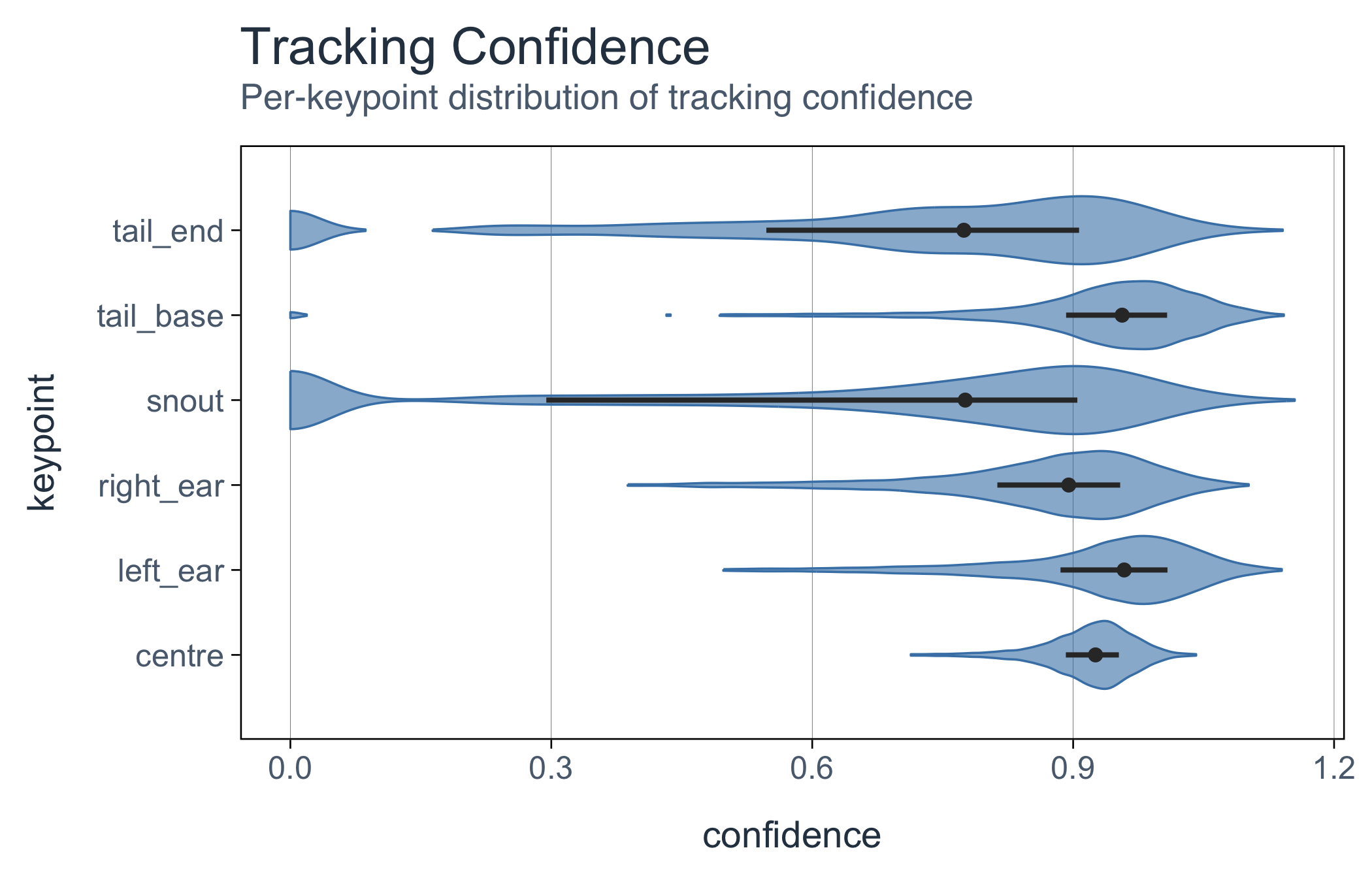
This is the plot to choose a threshold from. Most of each keypoint’s scores sit near 1, with a separate clump at zero and a thin spread in between, so a cut around 0.6 removes the failures without touching the good tracking. Where exactly to cut is a judgement about your data, and this plot lets you make it rather than guess.
Scores are whatever the tracker chose to emit. SLEAP’s run past 1 in this recording, and a 0.9 from one tool says nothing about a 0.9 from another. Read the distribution, rather than borrowing a threshold from someone else’s paper.
Missing values are the other half of the story. check_na_gapsize() reports how many there are and, more usefully, whether they come as short dropouts or long absences:
check_na_gapsize(movement)#>
#> -- Check: missing-value gap sizes
#> Tracking x: 9230 missing (8.3%) across 1019 gaps, longest 197 frames.
#> By group (individual and keypoint):
#> * individual1 | centre: 79 gaps, longest 108
#> * individual1 | left_ear: 87 gaps, longest 108
#> * individual1 | right_ear: 86 gaps, longest 108
#> * individual1 | snout: 331 gaps, longest 197
#> * individual1 | tail_base: 109 gaps, longest 108
#> * individual1 | tail_end: 327 gaps, longest 136The overall percentage hides the shape of the problem, and it differs a lot between keypoints. The snout and the tail end have hundreds of gaps each. The centre has far fewer, though its longest still runs to over a hundred frames. Plotting the centre on its own shows the shape:
movement |>
  dplyr::filter(keypoint == "centre") |>
  check_na_gapsize() |>
  plot()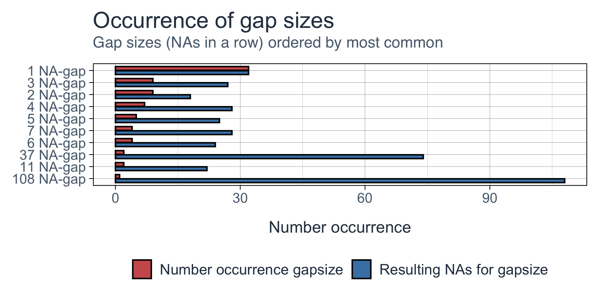
The difference matters for the next step. A gap of one frame is worth interpolating across, because the mouse can’t have gone far. A gap of a hundred frames is over three seconds, and anything drawn across it is invention.
These check plots put each group in its own panel, so with six keypoints you’ll want a taller figure (fig-height: 10 or so) before they become readable. One keypoint at a time is usually easier to read anyway.
Gaps clustered in one stretch mean something different from gaps spread evenly: a lighting change, say, rather than a keypoint the model was never good at. check_na_timing() splits the recording into intervals and shows how much of each is missing:
movement |>
  dplyr::filter(keypoint == "centre") |>
  check_na_timing() |>
  plot()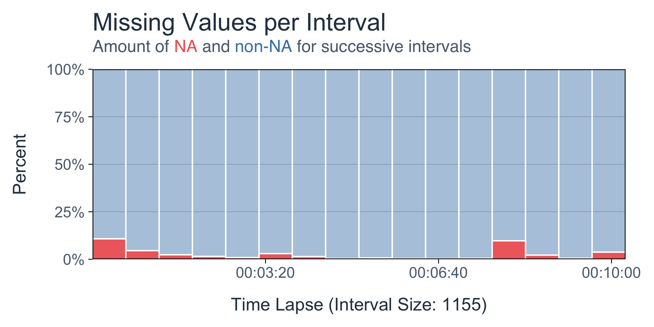
Very little of the centre is missing, with two worse patches: at the very start, and around seven and a half minutes in. Neither is a broken stretch of recording worth throwing away. They’re more likely moments when the mouse is hard to see, which is worth remembering when you interpret what it did then.
A mouse can’t stretch to twice its length between two frames, so a body segment whose length jumps around can point to a keypoint placed in the wrong spot. Using the skeleton the reader attached, check_segment_length() compares each segment’s length in every frame with its usual length:
check_segment_length(movement)#>
#> -- Check: segment lengths
#> Share of frames more than 30% off the reference length, for 7 segments of
#> structure "keypoint" (robust CV in brackets):
#> * individual1 | snout-left_ear: 42.0% [36.9%]
#> * individual1 | snout-right_ear: 37.4% [38.3%]
#> * individual1 | snout-centre: 0.5% [10.5%]
#> * individual1 | left_ear-centre: 13.6% [19.1%]
#> * individual1 | right_ear-centre: 12.0% [18.1%]
#> * individual1 | centre-tail_base: 2.6% [8.2%]
#> * individual1 | tail_base-tail_end: 4.8% [11.0%]plot(check_segment_length(movement))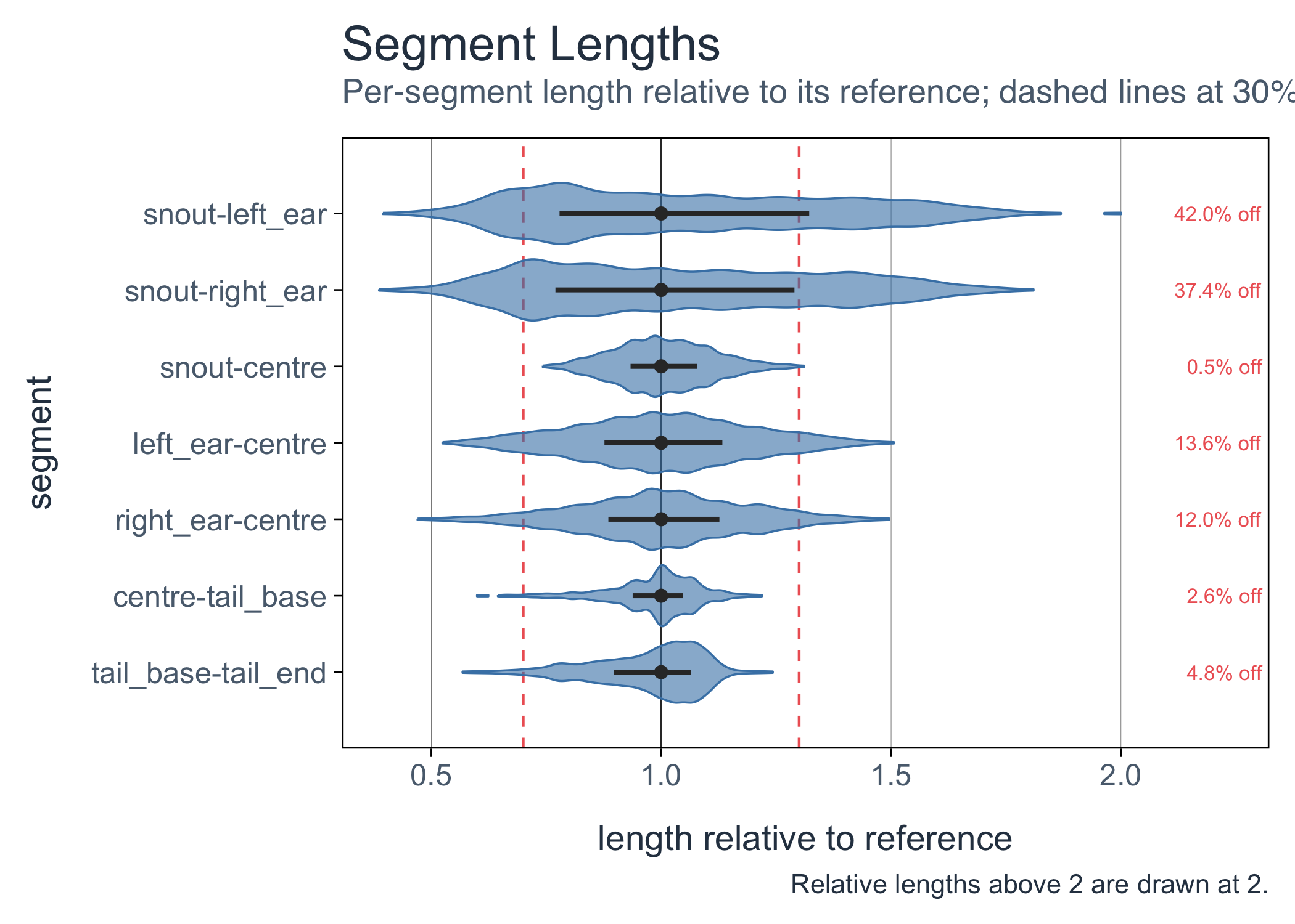
Read this with care in 2D. A camera looking down sees each segment’s length projected onto the floor, and that changes whenever the mouse rears, lowers its head or turns it. So segments vary in length even when the tracking is perfect. The short segments from the snout to the ears vary most, because a small movement of the head changes them by a large fraction. In 3D, where the true length is measured, the same check is much stricter. In 2D it is better at catching gross errors, such as two keypoints swapped, than at judging precision.
What the checks mean for the next guide:
Next: process the trajectories.