library(animovement)

clean <- read_dataset(get_sample_data("sleap")) |>
  set_metadata(sampling_rate = 30) |>
  convert_unit_time("s") |>
  convert_unit_space("cm", calibration_factor = 9 / 140) |>
  convert_unit_angle("deg") |>
  mask_na_across("roi", x_min = 19, x_max = 65, y_min = 0, y_max = 45) |>
  mask_na_across("confidence", threshold = 0.6) |>
  replace_na_across("linear", max_gap = 5) |>
filter_across("sgolay", window_width = 11, order = 3)Calculate metrics
Turn clean positions into speed, direction of travel, body heading and distance travelled, then summarise them.
Positions are rarely the answer to a research question. Speed, distance travelled, and how much an animal turned and when usually are. animetric derives them from a clean anipoint. We start from the pipeline in the previous guide, with one addition: angles in degrees rather than radians, which are easier to read.
Kinematics
add_kinematics() adds a column for each derived quantity. There’s nothing to configure: it reads the coordinate system, the sampling rate, the angle unit and the grouping from the metadata.
kinematics <- add_kinematics(clean)

setdiff(names(kinematics), names(clean))
#> [1] "speed" "acceleration" "cumulative_distance"
#> [4] "v_x" "v_y" "a_x"
#> [7] "a_y" "course" "course_unwrapped"
#> [10] "turning_speed" "turning_rate" "turning_acceleration"
#> [13] "cumulative_turning"The new columns come in two families:
- How fast:
speed,acceleration(how fast the speed changes),cumulative_distance(the distance travelled so far), and the velocity and acceleration along each axis,v_x,v_y,a_xanda_y. - Which way:
course, the direction of travel, and how it changes:turning_rate,turning_speed,turning_acceleration, andcumulative_turning.course_unwrappedis the same direction without the jump from 180° to −180°.
kinematics#> # Individuals: individual1
#> # Keypoints: centre, left_ear, right_ear, snout, tail_base, tail_end
#> # Sampling rate: 30 Hz
#> # Time: 00:00:00 to 00:10:16
#> individual keypoint time x y confidence speed acceleration
#> <fct> <fct> <dbl> <dbl> <dbl> <dbl> <dbl> <dbl>
#> 1 individual1 centre 0.0333 NA NA NA NA NA
#> 2 individual1 centre 0.0667 NA NA NA NA NA
#> 3 individual1 centre 0.1 NA NA NA NA NA
#> 4 individual1 centre 0.133 NA NA NA NA NA
#> 5 individual1 centre 0.167 NA NA NA NA NA
#> 6 individual1 centre 0.2 NA NA NA NA NA
#> 7 individual1 centre 0.233 NA NA NA NA NA
#> 8 individual1 centre 0.267 NA NA NA NA NA
#> 9 individual1 centre 0.3 NA NA NA NA NA
#> 10 individual1 centre 0.333 NA NA NA NA NA
#> # i 110,900 more rows
#> # i 11 more variables: cumulative_distance <dbl>, v_x <dbl>, v_y <dbl>,
#> # a_x <dbl>, a_y <dbl>, course <dbl>, course_unwrapped <dbl>,
#> # turning_speed <dbl>, turning_rate <dbl>, turning_acceleration <dbl>,
#> # cumulative_turning <dbl>A direction of travel only means something when the point actually moves. While the mouse sits still, tracking noise still moves its keypoints a fraction of a pixel, and the direction between two such positions is random. So below a minimum step, min_step, a row gets no course and adds nothing to the turning measures. By default it’s estimated from each track’s own noise, which is cautious. To be stricter, set it in the frame’s units, for example add_kinematics(clean, min_step = 0.1) for a millimetre.
ImportantCheck your units before you believe a number
Speed here is in centimetres per second, because we converted both units when reading the data. Every one of these numbers is only as good as those two conversions: get the sampling rate or the spatial scale wrong, and every speed is off by the same factor.
Look at it
plot_timeseries() draws a column against time:
kinematics |>
  dplyr::filter(keypoint == "centre") |>
  plot_timeseries(variable = "speed")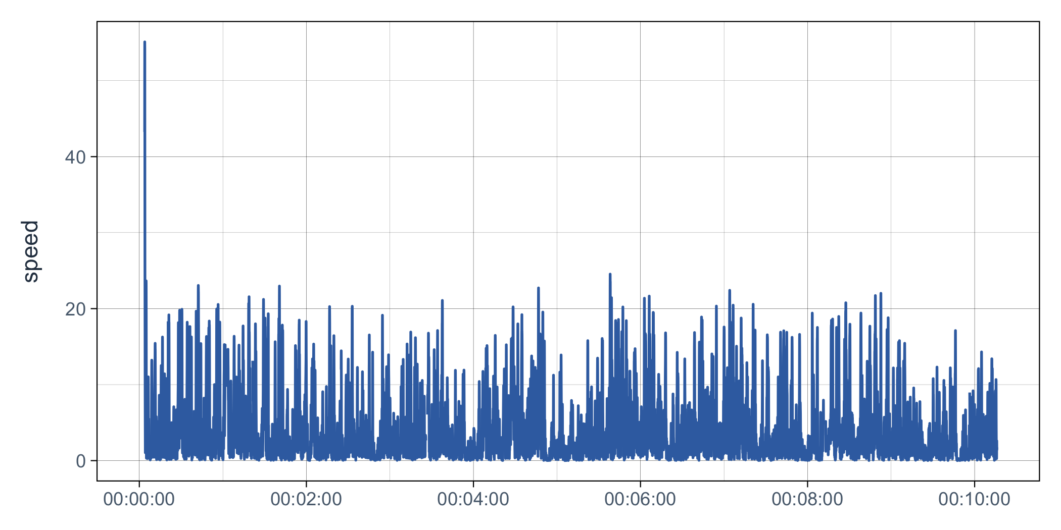
Bursts of movement separated by long still stretches: the pattern you’d expect from a mouse exploring a plus maze. A spike that looks too sudden to be real is worth going back to mask, with the "speed" or "hampel" method of mask_na_across(), rather than explaining away.
Where it goes and where it faces
course is the direction a point is moving. That isn’t always the direction the animal is facing: a mouse can turn its body while barely moving, and when it stops, there is no direction of travel at all.
Where the body points is its orientation, and add_orientation() works it out from two points. Here, the line from the base of the tail to the snout gives the mouse’s heading:
oriented <- clean |>
  add_orientation(from = "tail_base", to = "snout", level = "keypoint") |>
  add_kinematics()
The heading is attached to every keypoint, since it belongs to the body as a whole. Over one second of a run, the two directions start apart while the mouse turns, then come together as it runs straight:
oriented |>
  dplyr::filter(keypoint == "centre", time > 100, time < 101) |>
  dplyr::select(time, speed, course, heading)
#> # Individuals: individual1
#> # Keypoints: centre
#> # Sampling rate: 30 Hz
#> # Time: 00:01:40.033 to 00:01:40.967
#> individual keypoint time speed course heading
#> <fct> <fct> <dbl> <dbl> <dbl> <dbl>
#> 1 individual1 centre 100. 13.9 -173. -140.
#> 2 individual1 centre 100. 16.1 -170. -148.
#> 3 individual1 centre 100. 16.6 -168. -156.
#> 4 individual1 centre 100. 16.2 -169. -163.
#> 5 individual1 centre 100. 17.4 -171. -169.
#> 6 individual1 centre 100. 18.7 -172. -174.
#> 7 individual1 centre 100. 17.9 -173. -177.
#> 8 individual1 centre 100. 16.6 -177. -179.
#> 9 individual1 centre 100. 15.9 178. 180.
#> 10 individual1 centre 100. 14.2 174. 180.
#> # i 19 more rowsOver the whole recording, a circular plot shows where each direction points. Weighting course by speed lets the runs count for more than the shuffles:
centre <- dplyr::filter(oriented, keypoint == "centre")

plots(
  plot_circular(centre, variable = "course", weight = "speed"),
  plot_circular(centre, variable = "heading")
)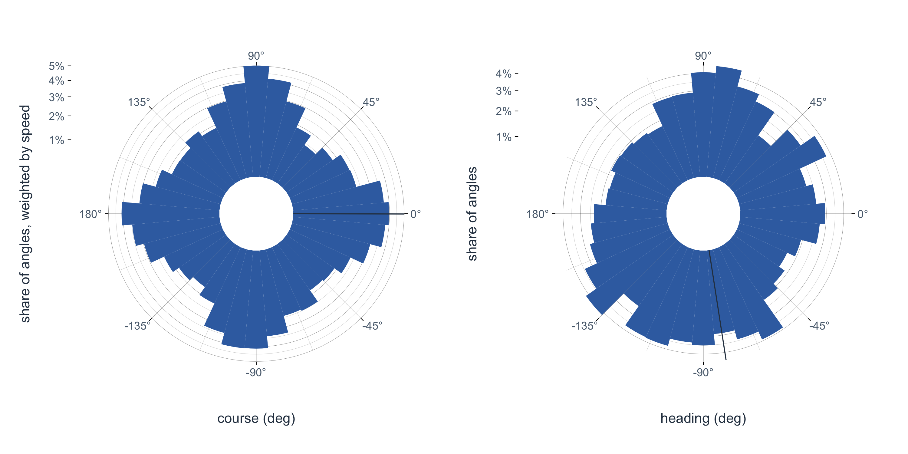
The direction of travel follows the four arms of the maze: that’s the only way to go. The body’s heading follows them too, but it also points along the diagonals, from the moments when the mouse sits nearly still and turns to look around. Those moments have no direction of travel at all, so only the heading can show them.
Summarise
Per-frame kinematics are the raw material; usually you want one row per track. animetric has two kinds of summary.
summarise_aniframe() summarises the distribution of each per-frame measure. It defaults to the median and the median absolute deviation (MAD), because movement data is rarely symmetric enough for a mean and standard deviation to describe it well. Angles such as course and heading get circular statistics, so the average of 350° and 10° comes out as 0°, not 180°.
summarise_aniframe(oriented)#> # A tibble: 6 x 18
#> individual keypoint median_speed mad_speed median_acceleration
#> <fct> <fct> <dbl> <dbl> <dbl>
#> 1 individual1 centre 2.55 2.44 0.0632
#> 2 individual1 left_ear 4.54 4.41 -0.210
#> 3 individual1 right_ear 4.58 4.39 -0.325
#> 4 individual1 snout 6.63 6.00 -0.857
#> 5 individual1 tail_base 2.54 2.62 -0.0641
#> 6 individual1 tail_end 2.19 2.69 0.0217
#> # i 13 more variables: mad_acceleration <dbl>, median_turning_speed <dbl>,
#> # mad_turning_speed <dbl>, median_turning_rate <dbl>, mad_turning_rate <dbl>,
#> # median_turning_acceleration <dbl>, mad_turning_acceleration <dbl>,
#> # median_confidence <dbl>, mad_confidence <dbl>, median_course <dbl>,
#> # mad_course <dbl>, median_heading <dbl>, mad_heading <dbl>There’s one row per keypoint, since that’s how this recording is grouped. The snout moves fastest: it swings as the mouse turns its head, so it covers more ground than the body it’s attached to. Pass measures = "mean_sd" if you’d rather have the mean and standard deviation.
summarise_path() describes each track’s path as a whole: the total distance, the total turning, how far the animal ended up from where it started, and how straight or winding the path was:
summarise_path(clean)#> # A tibble: 6 x 8
#> individual keypoint total_distance total_turning net_displacement straightness
#> <fct> <fct> <dbl> <dbl> <dbl> <dbl>
#> 1 individua~ centre 2510. 243452. 22.1 0.00880
#> 2 individua~ left_ear 3489. 201938. 20.0 0.00573
#> 3 individua~ right_e~ 3445. 203603. 14.0 0.00405
#> 4 individua~ snout 3135. 140416. 22.1 0.00704
#> 5 individua~ tail_ba~ 2420. 223257. 23.2 0.00960
#> 6 individua~ tail_end 2029. 211706. 5.33 0.00263
#> # i 2 more variables: sinuosity <dbl>, e_max <dbl>Beyond kinematics
The same anipoint feeds the rest of animetric:
add_point()adds a point derived from others, such as the centroid of the head from the snout and both ears.add_tortuosity()measures how winding a path is over sliding windows.calculate_nnd()finds the distance to the nearest neighbour, for recordings with several individuals.
When the question is about space rather than time, anispace transforms the coordinates themselves. transform_to_egocentric() re-expresses positions from the animal’s own point of view, map_to_polar() and related functions change the coordinate system, and rotate_coords() and translate_coords() align recordings with each other.
Where next
You’ve been through the whole workflow: read, check, process, measure. From here: